graph LR
    A[数据导入] --> B[数据清洗]
    B --> C[数据分析及可视化]
    C --> D[报告]
1 R 语言入门
R语言最初由Ross Ihaka和Robert Gentleman于1993年开发,是从S语言演变而来的开源编程语言。因其强大的数据处理和统计分析能力,R已成为数据科学领域的标准工具之一。
1.1 R在数据科学中的优势
- 丰富的统计与数据分析功能:内置众多统计分析函数,涵盖回归分析、时间序列分析、聚类分析等
- 强大的数据可视化能力:通过ggplot2等包可生成出版级质量的图表
- 广泛的社区支持与软件包生态:CRAN和Bioconductor提供数以万计的扩展包
1.2 数据分析流程
典型的数据分析流程如下:
常用分析包
readr:数据读取和保存tidyr:数据清洗dplyr:数据处理stringr:文本处理forcats:因子处理ggplot2:数据可视化
下面是一个完整的数据分析示例:
library(dplyr)
library(ggplot2)

# 生成示例数据
set.seed(123)
demo_data <- data.frame(
  x = rnorm(100),
  y = rnorm(100)
)

# 描述性统计
summary_stats <- demo_data |>
  summarise(
    mean_x = mean(x),
    mean_y = mean(y),
    sd_x = sd(x),
    sd_y = sd(y)
  )
print(summary_stats)
#> mean_x mean_y sd_x sd_y
#> 1 0.09040591 -0.1075468 0.9128159 0.9669866ggplot(demo_data, aes(x = x, y = y)) +
geom_point() +
labs(title = "Scatter Plot of x and y", x = "x", y = "y")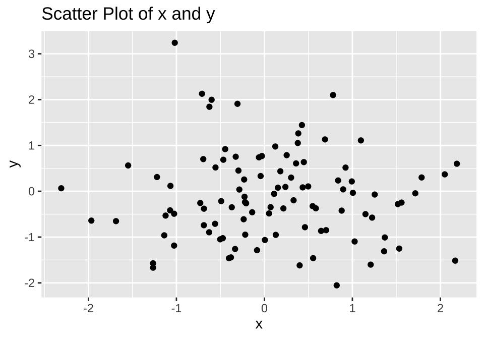
# 线性回归模型
model <- lm(y ~ x, data = demo_data)
summary(model)
#>
#> Call:
#> lm(formula = y ~ x, data = demo_data)
#>
#> Residuals:
#> Min 1Q Median 3Q Max
#> -1.9073 -0.6835 -0.0875 0.5806 3.2904
#>
#> Coefficients:
#> Estimate Std. Error t value Pr(>|t|)
#> (Intercept) -0.10280 0.09755 -1.054 0.295
#> x -0.05247 0.10688 -0.491 0.625
#>
#> Residual standard error: 0.9707 on 98 degrees of freedom
#> Multiple R-squared: 0.002453, Adjusted R-squared: -0.007726
#> F-statistic: 0.241 on 1 and 98 DF, p-value: 0.62461.3 基本概念与操作
1.3.1 数据类型与数据结构
1.3.1.1 向量、矩阵与数组
# 创建向量
numeric_vector <- c(1, 2, 3, 4, 5)
character_vector <- c("a", "b", "c", "d")
logical_vector <- c(TRUE, FALSE, TRUE, FALSE)

# 创建矩阵
matrix_example <- matrix(1:9, nrow = 3, ncol = 3)

# 创建三维数组
array_example <- array(1:24, dim = c(3, 4, 2))

print(numeric_vector)
#> [1] 1 2 3 4 5print(matrix_example)#> [,1] [,2] [,3]
#> [1,] 1 4 7
#> [2,] 2 5 8
#> [3,] 3 6 91.3.1.2 数据框与列表
# 创建数据框
data_frame <- data.frame(
name = c("Alice", "Bob", "Charlie"),
age = c(25, 30, 35),
city = c("New York", "Los Angeles", "Chicago")
)
# 创建列表
list_example <- list(
numeric_vector = numeric_vector,
matrix_example = matrix_example,
data_frame = data_frame
)
print(data_frame)#> name age city
#> 1 Alice 25 New York
#> 2 Bob 30 Los Angeles
#> 3 Charlie 35 Chicagoprint(list_example)#> $numeric_vector
#> [1] 1 2 3 4 5
#>
#> $matrix_example
#>      [,1] [,2] [,3]
#> [1,]    1    4    7
#> [2,]    2    5    8
#> [3,]    3    6    9
#>
#> $data_frame
#>      name age        city
#> 1   Alice  25    New York
#> 2     Bob  30 Los Angeles
#> 3 Charlie  35     Chicago
Note
数据框是R中最常用的数据结构,类似于数据库表格,可以包含不同类型的列。
1.3.1.3 因子与日期时间
# 创建因子
factor_example <- factor(c("Male", "Female", "Male", "Female"))
print(factor_example)
#> [1] Male Female Male Female
#> Levels: Female Male# 创建日期时间向量
date_time_vector <- as.POSIXct(c("2024-01-01 12:00:00", "2024-01-01 13:00:00"))
print(date_time_vector)#> [1] "2024-01-01 12:00:00 CST" "2024-01-01 13:00:00 CST"1.3.2 基本语法与操作
1.3.2.1 变量赋值与运算符
# 变量赋值
x <- 10
y = 20

# 比较运算
print(x == y)  # 等于
#> [1] FALSEprint(x != y) # 不等于#> [1] TRUEprint(x > y) # 大于#> [1] FALSE1.3.2.2 控制结构
# 条件判断
if (x > 0) {
  print("x is positive")
} else {
  print("x is negative")
}
#> [1] "x is positive"# for循环
for (i in 1:5) {
print(i)
}#> [1] 1
#> [1] 2
#> [1] 3
#> [1] 4
#> [1] 51.3.2.3 函数定义与调用
# 定义函数
my_function <- function(x) {
  return(x + 1)
}

# 调用函数
print(my_function(1))
#> [1] 21.4 数据分析软件包
1.4.1 dplyr包
1.4.1.1 数据筛选与过滤
data_frame |>
  filter(age > 30)
#> name age city
#> 1 Charlie 35 Chicago1.4.1.2 数据排序与汇总
# 排序
data_frame |>
  arrange(age)
#> name age city
#> 1 Alice 25 New York
#> 2 Bob 30 Los Angeles
#> 3 Charlie 35 Chicago# 汇总
data_frame |>
summarise(mean_age = mean(age))#> mean_age
#> 1 301.4.2 ggplot2包
Tip
ggplot2基于”图形语法”理论,通过层次化的方式创建图形。
1.4.2.1 基本用法
library(ggplot2)

# 创建示例数据
scatter_data <- data.frame(
  x = rnorm(100),
  y = rnorm(100),
  group = sample(letters[1:3], 100, replace = TRUE)
)

# 散点图
ggplot(scatter_data, aes(x = x, y = y, color = group)) +
  geom_point(size = 3, alpha = 0.7) +
  labs(title = "散点图示例", x = "X轴", y = "Y轴") +
  theme_bw()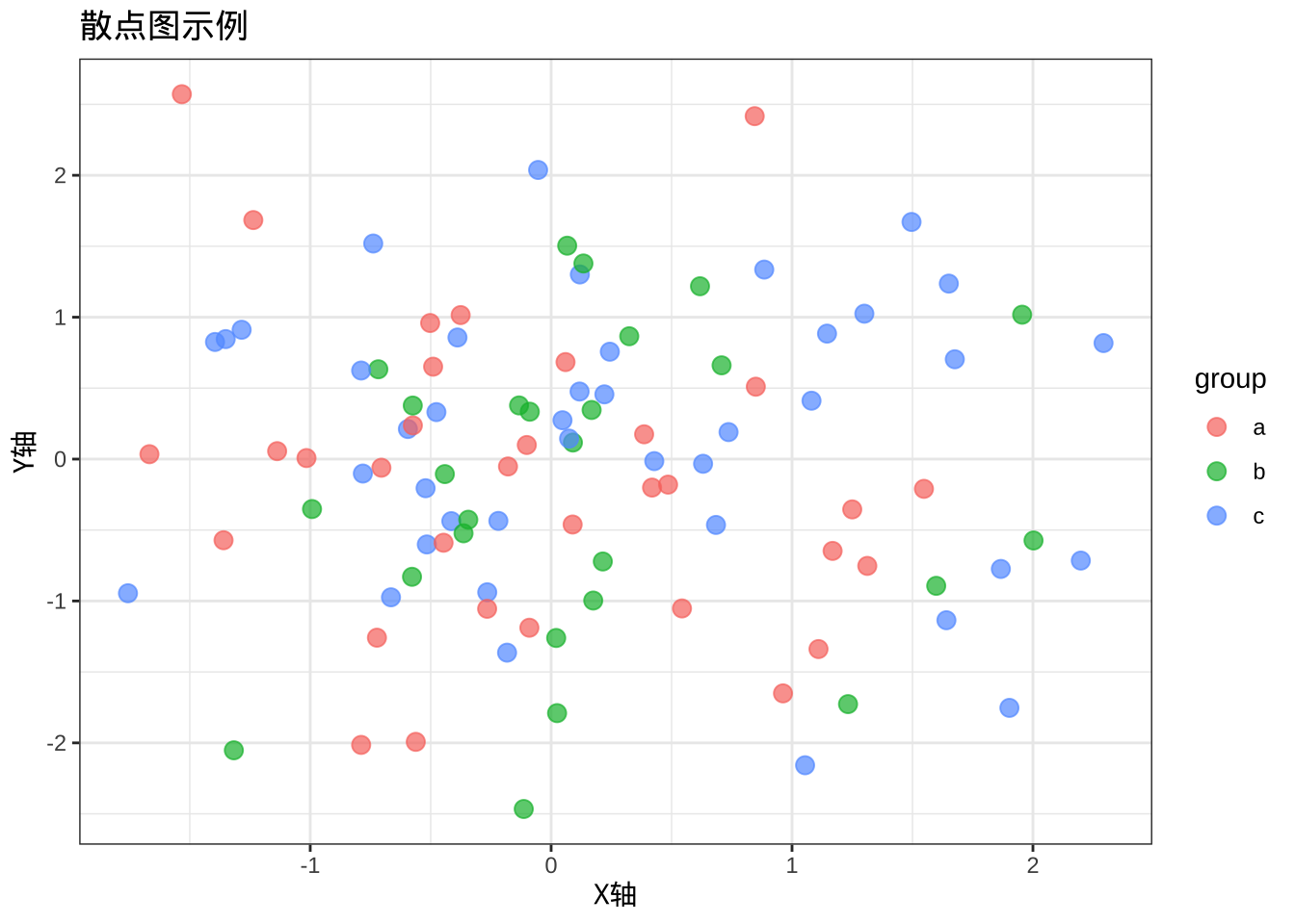
1.4.2.2 常见图表类型
# 折线图
time_data <- data.frame(
  time = 1:50,
  value = cumsum(rnorm(50))
)

p1 <- ggplot(time_data, aes(x = time, y = value)) +
  geom_line(color = "blue") +
  labs(title = "折线图") +
  theme_bw()

# 直方图
p2 <- ggplot(scatter_data, aes(x = x)) +
  geom_histogram(binwidth = 0.5, fill = "green", alpha = 0.6) +
  labs(title = "直方图") +
  theme_bw()

# 箱线图
p3 <- ggplot(scatter_data, aes(x = group, y = x, fill = group)) +
  geom_boxplot() +
  labs(title = "箱线图") +
  theme_bw()

cowplot::plot_grid(p1, p2, p3, labels = "auto", ncol = 3)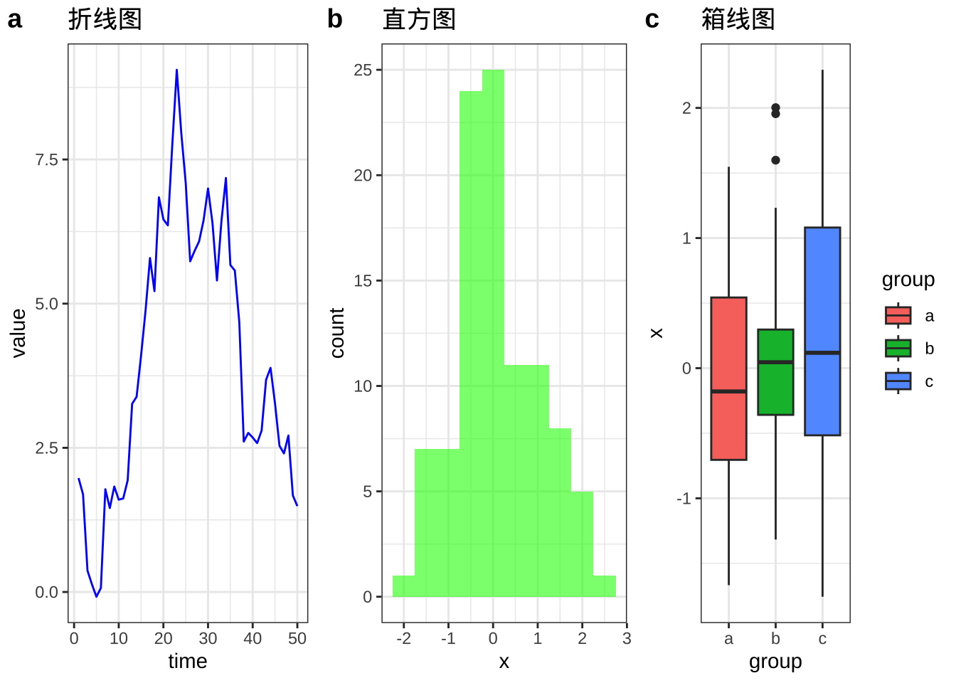
1.4.2.3 图层叠加
ggplot(scatter_data, aes(x = group, y = x, fill = group)) +
  geom_boxplot() +
  geom_jitter(aes(color = group), size = 3, width = 0.3, show.legend = FALSE) +
  labs(title = "箱线图叠加散点") +
  theme_bw()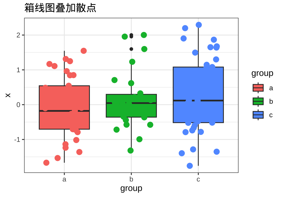
1.4.3 stringr包
library(stringr)

text <- "Hello, R language!"

# 提取子字符串
str_sub(text, 8, 9)
#> [1] "R "# 拼接字符串
str_c(text, " It's powerful!")#> [1] "Hello, R language! It's powerful!"# 替换字符串
str_replace(text, "language", "world")#> [1] "Hello, R world!"# 正则表达式匹配
text_vec <- c("apple123", "banana456", "cherry789")
str_detect(text_vec, "\\d+")#> [1] TRUE TRUE TRUEstr_replace_all(text_vec, "\\d+", "")#> [1] "apple" "banana" "cherry"1.4.4 tidyr包
library(tidyr)

# 创建宽格式数据
wide_data <- data.frame(
  ID = c(1, 2, 3),
  Math = c(90, 85, 88),
  Science = c(80, 78, 95),
  English = c(85, 89, 92)
)

# 宽转长
long_data <- wide_data |>
  pivot_longer(
    cols = Math:English,
    names_to = "Subject",
    values_to = "Score"
  )
print(long_data)
#> # A tibble: 9 × 3
#> ID Subject Score
#> <dbl> <chr> <dbl>
#> 1 1 Math 90
#> 2 1 Science 80
#> 3 1 English 85
#> 4 2 Math 85
#> 5 2 Science 78
#> 6 2 English 89
#> 7 3 Math 88
#> 8 3 Science 95
#> 9 3 English 92# 长转宽
wide_data_again <- long_data |>
pivot_wider(
names_from = Subject,
values_from = Score
)
print(wide_data_again)#> # A tibble: 3 × 4
#> ID Math Science English
#> <dbl> <dbl> <dbl> <dbl>
#> 1 1 90 80 85
#> 2 2 85 78 89
#> 3 3 88 95 92
Note
pivot_longer()和pivot_wider()是tidyr包的核心函数,分别用于宽长格式转换。这两个函数在数据清洗的时候作用很大,是必须要掌握的两个工具。
1.4.5 数据检查和清洗
# 创建含缺失值的数据框
data_with_missing <- data.frame(
  ID = c(1, 2, 3, 4),
  Name = c("Alice", "Bob", "Charlie", "David"),
  Score = c(95, NA, 88, 92)
)

# 检查缺失值
cat("各列缺失值数量:\n")
#> 各列缺失值数量:colSums(is.na(data_with_missing))#> ID Name Score
#> 0 0 1# 查看完整行
cat("\n完整行(无缺失值):\n")#>
#> 完整行(无缺失值):data_with_missing[complete.cases(data_with_missing), ]#> ID Name Score
#> 1 1 Alice 95
#> 3 3 Charlie 88
#> 4 4 David 92# 删除含缺失值的行
cat("\n删除缺失值后:\n")#>
#> 删除缺失值后:tidyr::drop_na(data_with_missing)#> ID Name Score
#> 1 1 Alice 95
#> 2 3 Charlie 88
#> 3 4 David 92# 填充缺失值(用均值填充)
cat("\n用均值填充缺失值后:\n")#>
#> 用均值填充缺失值后:data_with_missing |>
mutate(Score = ifelse(is.na(Score), mean(Score, na.rm = TRUE), Score))#> ID Name Score
#> 1 1 Alice 95.00000
#> 2 2 Bob 91.66667
#> 3 3 Charlie 88.00000
#> 4 4 David 92.00000
Note
处理缺失值的常用策略包括:删除含缺失值的行(drop_na())、用均值/中位数填充(replace_na())、或使用插值方法。选择哪种方法取决于缺失数据的比例和缺失机制。